Introduction/Background
That’s how much time an average American consumer spends on choosing what to watch next! With the amount of data we have today, we can be smarter and understand our options better. Every movie you watch has an official record that lets us know its rating, language, genre, cast, and a multitude of other details. Using this information, we aim to build a solution to make people’s lives easier!
Problem Definition
We formally divide our problem into two functional objectives, with the first one being -
“Recommend a set of similar movies to a user based on the movies they’ve watched before, or based on a particular movie they’ve searched.”
The method above is called content-based filtering - suggesting recommendations based on the item metadata. The main idea is if a user likes an item, then the user will also like items similar to it.
The other functional objective is -
“Suggest the top N movies to a user, based on other users with similar movie preferences.”
The method above is called collaborative filtering - these systems make recommendations by grouping users with similar interests.
Methods
Generally, Machine Learning projects evolve through a cycle of Data Cleaning, Preparation, Feature Generation & Selection, Modelling, Optimization & Deployment. As the process has become dynamic over time, a lot of these processes get supplemented with additional processes and tend to get iterative as well. For our project, we will use a few basic blocks or segments -
Data Collection
For one of the most critical steps in the pipeline, we used the MovieLens[1] dataset created by GroupLens Research (Department of CSE @UniversityOfMinnesota) which contains a multitude of data pertaining to movies. We decided to move ahead with the “MovieLens 25M.” owing to the variety of data and features. Released in December of 2019, it has a total of 25M ratings. 1M tags are applied to 62K Movies by almost 162K users.
For our functional objective, it was essential that we needed the data above, and some additional data that could help us get insights beyond the usual. Hence, we decided to scrape some data linked to the movies that were already in the “MovieLens 25M.” Dataset. We used the links.csv file to get tmdb_ids and scraped the data from the TMDB API, which was added to the collection of data we already had.
Data Cleaning & Preparation
Data Cleaning is an essential part of any data driven project. Working with large datasets means various types of data types like strings, booleans, numbers, currencies, date-time objects, etc., and it is important we pay close attention to how data is structured or populated. Sometimes, data is found to be duplicated, corrupted, present in different or invalid data types, structurally wrong, out of scale or even erroneous.
Above issues were dealt with by using following steps -
- Duplicate data was checked for using unique or primary features like
idandtitles, and if a duplicate row was found, it was dropped. - Later, each column was checked for missing data, and was handled as deemed appropriate for each feature. For reference, we used a roadmap offered by Alvira Swalin on this Medium Blog
- Similarly, we handled structural flaws or data errors by either correcting the data values & data types, or simply treating it as a missing datapoint.
Next, for preparation, it was important that we send our final data with adequately selected and standardized features, so that other learning tasks in the pipeline can be carried out with minimal or no issues. We followed the steps below -
- One of the ways to go about that is to normalize, scale or standardize the features, especially numerical.
- Once the features are standardized, we used Principal Component Analysis to identify the most relevant features.
Then, we packed all the updated data into a .csv file and pushed it further into the pipeline.
Data Exploration & Visualization
To understand and comprehend the data on a higher level is essential before process the data further and develop machine learning models. We explored the data and visualized a few things that were interesting.
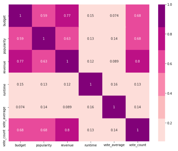
Here, in the first figure, we see a Correlation Matrix between the numerical variables of the tmdb_data dataset that offer information about the movies like budget,popularity,revenue,runtime,vote_average & vote_count. We observe that revenue and vote_count are highly correlated, but revenue and vote_average show weak correlation, which helps us understand that a big revenue movie may be reviewed by a lot of users, but it may not necessarily translate into a higher average rating. Similarly, revenue and budget also exhibit strong correlation.
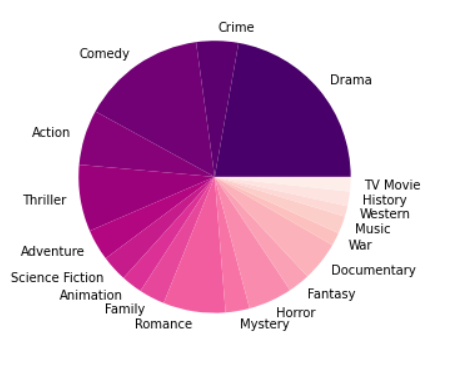
We also have a Pie Chart that breaks down the genres associated with all the movies, and the results follow the norm.
Files and Data
After the above steps, we have the following files that will help us solve our problems defined in the Problem Definition section -
movies.csvratings.csvtags.csvgenome-tags.csvgenome-scores.csvcredits-metadata.csvtmdb_data.csv
Learning Methods
We have implemented the following Supervised Learning methods in our project -
- Gaussian Naive Bayes
- Support Vector Machine
- Logistic Regression
- Random Forest Classifiers
- Decision Trees
- K-Nearest Neighbors
- Matrix Factorization using Neural Networks
In addition, we have implemented the following Unsupervised Learning methods -
- Association Rules using Apriori
- Content-based filtering
- TF - IDF matrix
- Cosine similarity
- Collaborative filtering
- Matrix factorization using Singular Value Decomposition (SVD)
Supervised Learning
To predict movie ratings using user data, we implemented a few Supervised Learning algorithms, with the training set structured as follows:
Features : movie_id, age, occupation
Label: rating
These algorithms gave out accuracies as below -
| Model | Accuracy |
|---|---|
| Gaussian Naive Bayes | 35.89 |
| Support Vector Machine | 35.27 |
| Logistic Regression | 33.93 |
| Random Forest | 30.17 |
| Decision Trees | 28.29 |
These algorithms offered subpar accuracies which weren’t acceptable. So, we decided to move to Matrix Factorization to solve the rating prediction problem.
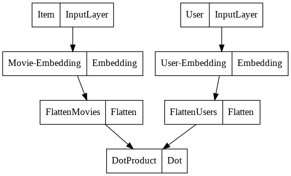
Matrix Factorization using Neural Networks
Matrix factorization is a simple embedding model. In the context of our project: Given the Ratings Matrix A of dimensions m * n, where m is the number of users and n is the number of movies, the model learns -
- A user embedding matrix U of dimesnions
m * d, where row i is the embedding for user i. - A movie embedding matrix V of dimensions
n * dwhere row j is the embedding for item j.
The embeddings are learnt such that the product U.VT is a good approximation of the Ratings Matrix A. The (i, j) entry of U.VT is simply the dot product <UiVj> of the embeddings of user i and item j, which you want to be close to Aij.
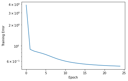
For the purpose of our project, we have set the number of latent factors to be 20 and have made use of two objective functions, namely Mean Absolute Error (MAE) and Mean Squared Error (MSE).
The following figures depict the model architecture being used and a graph representing the training loss v/s number of epochs.
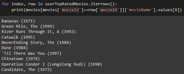
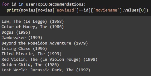
Here are the results obtained by using Matrix Factorization. The first image shows us a sample user’s top 10 rated movies. The second image shows us the recommendations given by our model. As we can see, the results seem to be in line with the user’s choice and liking.
Item-Based Collaborative Filtering
The main idea of this approach is to find similar movies instead of similar users. This can be explained with the following example : take two movies, A and B, and check their ratings by all users who have rated both movies. If these ratings are similar, it’s highly probable that the two movies are similar, so someone who liked movie A would also probably like movie B, and vice versa. This is calculated for every pair of movies rated by each user, and takes both user and movie understanding into account while recommending new movies - giving us a hybrid between the content-based and collaborative methods, which will be discussed later.
One of its advantages over user-based collaborative filtering, is that movies, unlike people’s opinions, don’t change over time. So by finding similarity between movies rather than users, we can be sure our recommendations hold good over time. Also, there are much fewer movies in comparison to users, so finding the pairwise calculations of movies would still be less resource intensive.
Implementation Details: We start with some data filtering to ignore movies that have less than 10 ratings as it wouldn’t be credible enough, and also users that have rated less than 50 movies. We want to reduce the sparsity of our data. We use the K-Nearest Neighbors algorithm in this approach, to compute similarities between movies based on their cosine distances. When a user inputs a movie name, we can use KNN to rank the similarities of movies and display the 10 closest outputs.
Unsupervised Learning
Content-Based Filtering
This algorithm is used to compute similarities between movies based on certain metrics (we experiment with different combinations of these metrics). The idea is to recommend movies based on a particular movie that the user liked (taken as an input).
The first category is movie description. Here, we experimented with all possible combinations of : overview (plot), tagline and genre.
We found the overview and genres to be highly useful, but the tagline not so much, so we went ahead with a feature set of words from the overview + genre in the next stage of the pipeline. We build the TF-IDF matrix using these words, to find the relevance of each word to each movie. Stop words have been accounted for, and are filtered out of the feature list. We use the cosine similarity score to find the similarity between each pair of movies. Then, based on the movie input by the user, we can get the N most similar movies using this score.
Some examples of the recommendations based on overview :
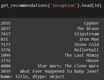
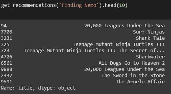
It’s quite obvious that these recommendations have been made solely based on the movie descriptions, without looking at extra information like the cast and crew, or popularity of the movie and other user’s ratings.
To take content-based filtering to the next step, we look at the movie metadata - including the cast, crew and keywords about the movie. From the crew, we take only the director as our feature for now, however this will be extended in the future. There are several other departments to take into consideration like Writing, Director of Photography, Sound Design / Music, Screenplay, etc. and based on which is the most important to a user, we can weigh it accordingly. For the cast, we take the top three names from the credits list, as these correspond to the major characters. However, some users still watch movies regardless of the size of the role of their favorite actor, so this can also be considered in the weighting process. For example, the director has been weighted thrice as much as other cast members, so it is given more priority.
Coming to the keywords, we do a basic frequency based filtering to remove those words that occur only once. This is followed by stemming, which refers to the process of reducing each word to its root, without its suffixes or prefixes (called the lemma). Eg. “run” and “running.” are considered the same word since they have the same meaning with respect to the plot.
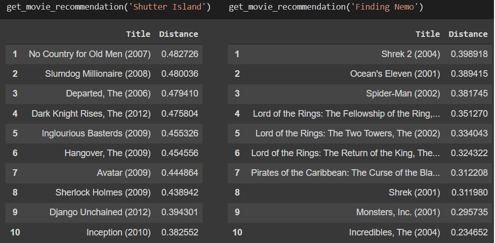
Some examples of the recommendations after taking into account the metadata :

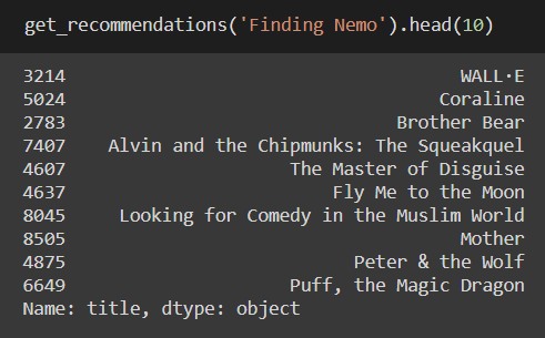
It does a much better job! Some further experiments we can perform in the future including weighting based on crew, actors, genre, or other features like language.
Optimization
Applying PCA on BERT embeddings
We first transform the sentences of the overview feature into BERT embeddings. The dimension of the embeddings in our code comes out to be 768. We then run PCA on the obtained BERT embeddings to carry out dimensionality reduction. The resultant reduced dimension of the embeddings comes out to be 60. The explained variation per principal component is 0.897.
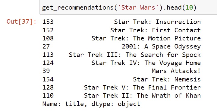
After running PCA on our BERT embeddings, we run a cosine similarity measure on the obtained matrix instead of the TF - IDF matrix that was used in the initial content based filtering approach. We observe improved results as can be seen from the figure below:
User-Based Collaborative Filtering
The content-based filtering algorithm solely takes into consideration the movie information, and nothing about the personal taste of the user while giving suggestions. Hence, every user would be recommended the same set of movies, regardless of who they are and what they like. Hence, we bring in collaborative filtering, which suggests movies to a user based on what other users with similar preferences have enjoyed watching. We use a dataset of user ratings for this algorithm, which correspond to our movie database dataset.
We use the Surprise library, which uses Singular Value Decomposition to compute accuracy measures like Root Mean Square Error and Mean Absolute Error, using a k-fold cross-validation procedure (in our case, 5-fold).
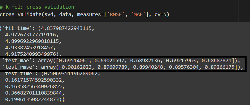
As we can see, we get an average Root Mean Square Error of about 0.896. We can then go ahead with the training and predictions.
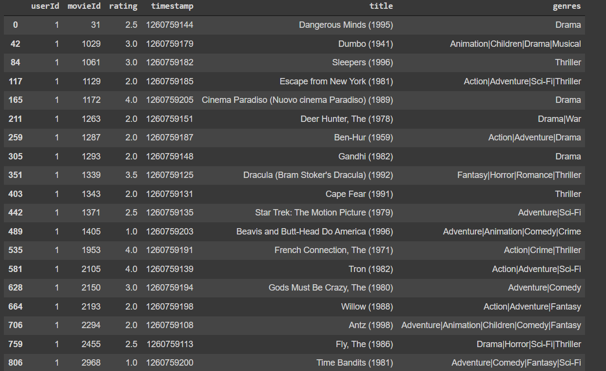
Here’s an example of a user (with userId 1) and all the movies they have rated. It seems like this user is more inclined towards Thriller or Action based movies, and not so much inclined towards Comedy or Animation.
We run our algorithm to predict how this user would rate a new movie, and this is based on how other users with similar preferences have rated that movie.
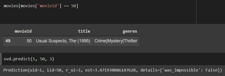
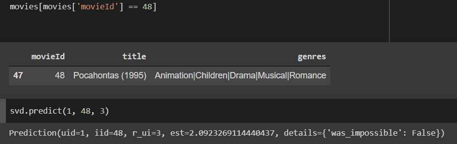
We can see that the user rating prediction for The Usual Suspects is a 3.47, while the prediction for Pocahontas is a 2.09. This is in line with the earlier observation, as The Usual Suspects is more of a Thriller and Mystery, while Pocahontas is more of an Animation and Musical.
Some of the disadvantages of the user-based collaborative filtering approach are that it’s purely based on personal opinion which could keep changing. Even if two users had similar preferences at one point, it might not stay the same over time. Furthermore, there are way more users than movie items and it becomes difficult to recompute these large matrices regularly.
This motivated us to explore a better method called item-based collaborative filtering, which was discussed in the supervised learning section earlier.
Apriori
Apriori, is an association rule mining algorithm often used in frequent item set mining. The most important application of this algorithm is Market Basket Analysis, helping customers in purchasing based on their shopping trends. The most recent usage of Apriori is recommendation systems and hence the reason for implementation.
Support
The model is used to calculate the probability and helps determine the likelihood of a user to watch movie M2 when he has already watched movie M1. This is computed by calculating support, confidence and lift for a variety of movie combinations.
Support is calculated for M1 movie using the following formula:
Support(M1) = (# users watch lists containing M1) / (#user watch lists)
So, support calculates, the percentage of users with movie M1 in their watch lists out of all the users
Confidence
The confidence value of a certain movie is the percentage of users who have watched both M1 and M2 out of users whose watch lists contain M1 and confidence is denoted as Confidence (M1 -> M2) and the formula is:
Confidence (M1 -> M2) = (# users watch lists with M1 and M2) / (# users with M1 in their watch lists)
Essentially, confidence is the measure of the likelihood of users watching M2 if it is recommended to users who have already watched M1 (subset of the population)
Lift
The measure of the increase in likelihood of movie M2 being watched by users who watched M1 over its likelihood when recommended to the entire population. The higher the value of the lift, more likely it is for users to watch M2 when recommended to users with M1 in their watch lists. The formula is
Lift ( M1 -> M2) = Confidence (M1 -> M2) / Support (M2)
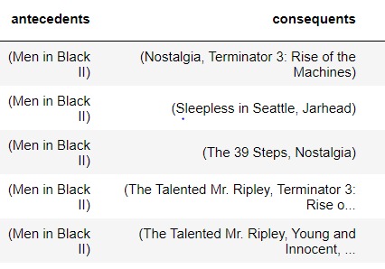
The antecedents are the movies watched and consequents are the suggested movies using Apriori:
Hybrid
Hybrid recommender systems implements both content and collaborative filtering methods. This often proves to be more effective and can be implemented in several ways:
- Combining predictions from content-based and collaborative-based methods
- Using content-based capabilities in a collaborative-based approach
- Using collaborative-based capabilities in a content-based approach
LightFM[8] is a hybrid matrix factorization model representing users and items as linear combinations of the latent factors of their content features. Similar to collaborative filtering, users and items are represented as embeddings. Just as in a Content Based model, these are entirely defined by functions (linear combinations) of embeddings of the content features that describe each user.
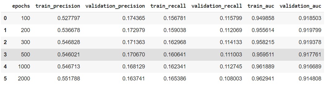
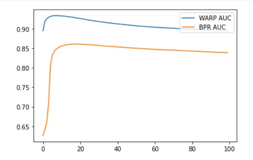
LightFM implements the WARP (Weighted Approximate-Rank Pairwise) loss for implicit feedback learning-to-rank. Usually, it is better in peformance than the BPR (Bayesian Personalised Ranking) loss by a large margin. Comparing two models with equivalent hyperparameters and compare their accuracy across epochs. We are using Precision & Recall for top-10 recommendations. We used 100 Epochs, 50 components (dimensionality of feature latent embedding), and AdaGrad learning grade schedule.
After plotting the results it is revealed that WARP produces superior results. Test accuracy decreases after the first 10 epochs, suggesting WARP starts overfitting and would benefit from regularisation or early stopping.

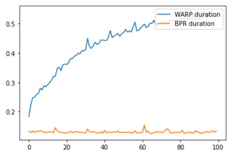
WARP is slower than BPR for all epochs.
Also, LightFm performs considerably well in case of Cold Starts (new users and items) with the use of user and item metadata. It also deals with sparsity pretty well, giving out decent recommendations.
Timeline
Since the project expects multiple stages and processes, the team members will collaborate on each section to ensure timely delivery of the module, reduced error probability, and a good learning experience. Our members will use tools and services like GitHub, LiveShare, etc. to ensure that they are actively working on ideation and implementation. Bigger sections will be broken into smaller phases and will be taken over by all the members in multiple chunks. The whole project timeline will consist of such phases, are detailed as below -
| Process/Stage | Date Range |
|---|---|
| Data Collection, Cleaning & Preparation | 10/05 - 10/25 |
| Feature Creation & Selection | 10/25 - 11/05 |
| Modelling (Unsupervised) | 11/05 - 11/16 |
| Modelling (Supervised) | 11/16 - 11/25 |
| Optimization & Tuning Parameters | 11/25 - 11/28 |
| Implementing Final Modules & Models | 11/28 - 12/01 |
| Final Proposal & Presentation | 12/01 - 12/07 |
Results and Discussions
We decided to use Matrix factorization as our first approach for recommending movies to a user. In order to learn the embeddings, we first need to calculate a ratings matrix for the users. It is not possible that every user would have watched every single movie, so we first need to predict the ratings a user might give a movie. After trying a few supervised learning algorithms such as Random Forest, Logistic Regression, Support Vector Machines, etc. for predicting the ratings, we decided to move forward with the combination of neural networks and matrix factorization for making our initial movie recommendations.
To get similarities between different movies and make recommendations based on similar movies, we decided to give content-based filtering a try, wherein the algorithm uses certain metrics such as overview and genre to output similar movies based on a particular input. After initially just transforming the metrics into BERT embeddings, we ran PCA to reduce the dimensions of these embeddings from 768 to 60. A drawback with this approach was that content based filtering does not take into consideration anything about the personal taste of the user, so it would recommend the same set of movies to every set of users. To overcome this, we moved onto collaborative filtering where we suggest movies to a user based on what other users with similar preferences like. These user preferences are used to predict ratings for a movie the user hasn’t seen and then decide if the user would enjoy watching that movie. We did get decent results and favorable predictions for user-based collaborative filtering but realized that such an approach is highly dependent on personal opinion which might change over time and recalculating such large matrices before every prediction is not feasible. This led to us exploring the item-based filtering approach, where we try to find similar movies, instead of basing our decision only on similar users. Because movies don’t change over time like user opinions, these predictions have a much higher chance of holding good over time, while being much less resource intensive. When a user inputs a movie, we use k-nearest neighbors algorithm to compute similarities between movies and output the top closest ones.
Our next approach was Apriori, which was much more comprehensive in nature. Apriori makes recommendations by measuring the increase in likelihood of a movie being watched by users given that they have watched another movie, over its likelihood when that movie is recommended to the entire population. These two calculated features are known as support and confidence respectively.
The final approach that we tried was a hybrid one, which combined both content and collaborative based models. We used LightFM as the hybrid matrix factorization method to achieve this. Unlike previous methods, this ensures that both the user as well as the item metadata are taken into consideration in both cold-start or sparse interaction data scenarios. User and item data are converted to embeddings and represented as linear combinations of the latent factors of their content features. This model clearly outperforms the previously implemented ones as can be seen from the metrics above, and also the associated movie recommendations.
References
-
F. Maxwell Harper and Joseph A. Konstan. 2015. The MovieLens Datasets: History and Context. ACM Trans. Interact. Intell. Syst. 5, 4, Article 19 (January 2016), 19 pages. DOI:https://doi.org/10.1145/2827872
-
“Recmetrics.” PyPI, https://pypi.org/project/recmetrics/
-
Kumar, Manoj, et al. “A movie recommender system: Movrec.” International Journal of Computer Applications 124.3 (2015).
-
Cintia Ganesha Putri, Debby, Jenq-Shiou Leu, and Pavel Seda. “Design of an unsupervised machine learning-based movie recommender system.” Symmetry 12.2 (2020): 185.
-
Chen, Hung-Wei, et al. “Fully content-based movie recommender system with feature extraction using neural network.” 2017 International Conference on Machine Learning and Cybernetics (ICMLC). Vol. 2. IEEE, 2017.
-
Cui, Bei-Bei. “Design and implementation of movie recommendation system based on Knn collaborative filtering algorithm.” ITM web of conferences. Vol. 12. EDP Sciences, 2017.
-
Katarya, Rahul, and Om Prakash Verma. “An effective collaborative movie recommender system with cuckoo search.” Egyptian Informatics Journal 18.2 (2017): 105-112.
-
Maciej Kula (2015). Metadata Embeddings for User and Item Cold-start Recommendations. In Proceedings of the 2nd Workshop on New Trends on Content-Based Recommender Systems co-located with 9th ACM Conference on Recommender Systems (RecSys 2015), Vienna, Austria, September 16-20, 2015. (pp. 14–21). CEUR-WS.org.